I had created two different clusterings, and my colleague Adam Reid suggested that I create a 'riverplot' (see here for a nice description) to show the overlaps between the clusters in clustering RUN1, and clustering RUN2 (made from two different runs of the same clustering software, with slightly different inputs).
To do this, I used the riverplot R package.
For my clusterings RUN1 and RUN2, I had found overlaps between the clusters in set RUN1, and the clusters in set RUN2, as follows, where (x, y) gives the number of overlaps between a cluster x in set RUN1 and a cluster y in set RUN2:
- pair (5, 4) : 15005
- pair (6, 5) : 5923
- pair (4, 4) : 4118
- pair (0, 3) : 9591
- pair (4, 5) : 3290
- pair (5, 5) : 17
- pair (1, 0) : 13890
- pair (3, 2) : 4131
- pair (2, 3) : 504
- pair (2, 1) : 16480
- pair (0, 0) : 1
- pair (0, 1) : 4
- pair (1, 2) : 62
- pair (4, 0) : 6
- pair (3, 3) : 135
- pair (2, 4) : 113
- pair (3, 1) : 43
- pair (1, 1) : 17
- pair (3, 4) : 64
- pair (1, 4) : 6
- pair (4, 3) : 148
- pair (0, 5) : 38
- pair (1, 3) : 16
- pair (2, 2) : 12
- pair (0, 2) : 2
- pair (5, 3) : 15
- pair (6, 4) : 40
- pair (0, 4) : 14
- pair (6, 3) : 3
- pair (1, 5) : 2
- pair (4, 1) : 5
- pair (4, 2) : 1
- pair (2, 0) : 2
- pair (5, 0) : 2
You could I guess show this as a weighted graph, ie. with nodes in RUN1 on the left and nodes in RUN2 on the right, and edges between them, with the weight for each edge written on it.
Another nice way is a riverplot. I made this using the riverplot package as follows:
> install.packages("riverplot")
> library("riverplot")
> nodes <- c("RUN1_0", "RUN1_1", "RUN1_2", "RUN1_3", "RUN1_4", "RUN1_5", "RUN1_6", "RUN2_0", "RUN2_1", "RUN2_2", "RUN2_3", "RUN2_4", "RUN2_5")
> edges <- list( RUN1_0 = list( RUN2_0=1, RUN2_1=4, RUN2_2=2, RUN2_3=9591, RUN2_4=14, RUN2_5=38),
+ RUN1_1 = list( RUN2_0=13890, RUN2_1=17, RUN2_2=62, RUN2_3=16, RUN2_4=6, RUN2_5=2),
+ RUN1_2 = list( RUN2_0=2, RUN2_1=16480, RUN2_2=12, RUN2_3=504, RUN2_4=113, RUN2_5=0),
+ RUN1_3 = list( RUN2_0=0, RUN2_1=43, RUN2_2=4131, RUN2_3=135, RUN2_4=64, RUN2_5=0),
+ RUN1_4 = list( RUN2_0=6, RUN2_1=5, RUN2_2=1, RUN2_3=148, RUN2_4=4118, RUN2_5=3290),
+ RUN1_5 = list( RUN2_0=2, RUN2_1=0, RUN2_2=0, RUN2_3=15, RUN2_4=15005, RUN2_5=17),
+ RUN1_6 = list( RUN2_0=0, RUN2_1=0, RUN2_2=0, RUN2_3=3, RUN2_4=40, RUN2_5=5923))
> r <- makeRiver( nodes, edges, node_xpos = c(1, 1, 1, 1, 1, 1, 1, 2, 2, 2, 2, 2, 2), node_labels=c(RUN1_0 = "0", RUN1_1 = "1", RUN1_2 = "2", RUN1_3 = "3", RUN1_4 = "4", RUN1_5 = "5", RUN1_6 = "6", RUN2_0 = "0", RUN2_1 = "1", RUN2_2 = "2", RUN2_3 = "3", RUN2_4 = "4", RUN2_5= "5"), node_styles= list(RUN1_0 = list(col="yellow"), RUN1_1 = list(col="orange"), RUN1_2=list(col="red"), RUN1_3=list(col="green"), RUN1_4=list(col="blue"), RUN1_5=list(col="pink"), RUN1_6=list(col="purple")))
> plot(r)
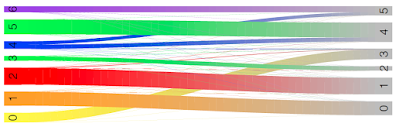
Here we see cluster 0 in RUN1 mostly corresponds to cluster 3 in RUN2.
Cluster 1 in RUN1 mostly corresponds to cluster 0 in RUN2.
Cluster 2 in RUN1 mostly corresponds to cluster 1 in RUN2.
Cluster 3 in RUN1 mostly corresponds to cluster 2 in RUN2.
Clusters 4,5,6 in RUN1 correspond to clusters 4 and 5 in RUN2: cluster 4 in RUN2 maps to clusters 5 and 4 in RUN1, and cluster 5 in RUN2 maps to clusters 6 and 4 in RUN1.
Note in some cases you might have a lot of clusters, then you can reduce down the label size for the clusters as described here ie.:
> custom.style <- riverplot::default.style()
> custom.style$textcex <- 0.1
> plot(r, default_style=custom.style)
Acknowledgements
Thanks to Adam Reid for introducing me to riverplots!

