Thursday 20 December 2012

Using gap5 to view SAM/BAM files

The Gap5 program by James Bonfield and Andrew Whitwham is part of the Staden package, and can be used to view reads that are aligned to a genome assembly (in SAM/BAM format), and to edit the genome assembly.

Gap5 is very useful if you want to have a quick look at reads aligned to a part of a genome assembly. For example, say we have our read-to-genome stored in a BAM file 'my.bam', then we can extract reads aligning to positions 11000-13000 of scaffold 'myscaffold' by typing:
% samtools index my.bam my.bam.bai 
% samtools view my.bam myscaffold:11000-13000 > my.sam
The first line indexes the BAM file so we can pull subsets of data from it. The second line makes a sam file my.sam containing the reads aligning to positions 11000-13000 of 'myscaffold'.

We can then make a Gap5 database file out of the SAM file my.sam by typing:
% /Users/alc/Documents/Software/Staden2.0.0b9/bin/tg_index my.sam
where /Users/alc/Documents/Software/Staden2.0.0b9/bin/tg_index is the path to the 'tg_index' program within the installed Staden package (note that this path may differ on your computer, depending on where you installed the Staden package).
   This makes files my.0.g5d and my.0.g5x, which are the Gap5 database files.

To start up Gap5, you double-click on the Gap5 icon within the installed Staden package (eg. in directory 'Staden2.0.0b9'). This starts up Gap5, and brings up the main window.


You can select 'my.0.g5d' by going to the File menu, and choosing 'Open' and then choosing the my.0.g5.d file. This will bring up the 'Contig selector' which has your contigs (in this case just one contig 'myscaffold'):
To view the reads aligned to a contig/scaffold, in the main window, go to the 'View' menu and choose 'Template Display', then choose your contig/scaffold of interest. This will bring up a picture of the contig/scaffold with the aligned reads:
In this case, there are quite few reads, so they are hard to distinguish from the white horizontal line.

To view the alignments of individual reads, click on the white horizontal line. This brings up a view of the alignments of individual reads:
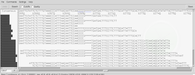

There are two scroll-bars across the bottom. The top one lets you move shorter distances, and the bottom one lets you move large distances. In the line at the top of the screen you can see the consensus sequence inferred for the genome sequence by Gap5, based on the read alignments.

By default, soft-clipped bases are not shown. If you tick the 'Cutoffs' box at the top of the window, they will be shown in pale grey.

Another useful thing to know is that by default, Gap5 gives 'padded coordinates', meaning that extra bases are inferred in the genome sequence (based on the reads) that were not in the original fasta file of scaffolds that the reads were aligned to, to make BAM file. In other words, in some cases, all the reads aligning at a position have an extra base that wasn't in the original fasta file, so this gives an extra base position in the consensus inferred by Gap5 at the top of the window. If you want to see the original reference genome coordinates (ie. coordinates with respect to the original fasta file of scaffolds) instead of the padded coordinates, go to the 'Settings' menu, and choose 'Reference coordinates'.

Thanks to Alan Tracey for introducing me to Gap5, a very nice tool.

Cigar alignments and insert sizes in SAM/BAM format

The alignments in a SAM/BAM file are stored in 'cigar' format, in which 'M' means a match or mismatch, 'I' means an insertion in the read relative to the reference genome, and 'D' means a deletion in the read relative to the reference genome.

For example, the alignment:
ACTGATTTGG- (genome)
|||||   ||
AATGA---AGT (read)
has cigar string 5M3D2M1I.

Bases at the start or end of a read may be 'soft-clipped' (usually because they are low quality sequence). This can be represented as 'S' in the cigar string. For example, the alignment:
ACTGATTTGG- (genome)
   ||   ||
AATGA---AGT (read)
in which the read bases have been soft-clipped, has cigar string 3S2MD2M1I.

Column 4 of a SAM/BAM file is the mapped position of a read. This contains the position of the reference genome that the first non-softclipped base of the read is mapped to (according to the SAM format specification). That is, it ignores soft-clipped bases at the start of the read. Therefore, if you soft-clip more bases at the start, you must change column 4.
       For example, the following alignment has cigar '3S2M3D2M1I' and start position 100:
ACTGATTTGG- (genome)
   ||   ||
AATGA---AGT (read)
If we soft-clip another base at the start of the alignment, we get cigar '4S1M3D2M1I' and start position 101:
ACTGATTTGG- (genome)
    |   ||
AATGA---AGT (read)

Column 8 of a SAM/BAM file is the mapped position of the mate. Therefore, if we changed the mapped position of a read x (by soft-clipping) as above, we must then change column 8 of the SAM/BAM for the mate of read x.

Column 9 of a SAM/BAM file has the inferred insert size of a read-pair. According to the SAM format specification this is defined by the first position of mapped position of the first read and the last mapped position of the second read (ignoring soft-clipped bases) of a read-pair. Therefore, if we changed the mapped position of a read x (by soft-clipping) as above, we must change column 9 of the SAM/BAM for read x and for the mate of read x.

For example, if you have:
read x: start-position: 144558, cigar: '5S95M'
mate of read x: start-position: 147480, cigar '2S98M'
The left-most mapped base of read x is base 144558 in the reference.
The right-most mapped base of the mate of read x is 147480 + (sum of M/D/N operations in the cigar for the mate of read x) - 1 = 147480 + 98 - 1 = 147577 in the reference.
Therefore, the insert size = 147577 - 144558 + 1 = 3020 bp.

Thanks to my colleague Martin Hunt for discussion. 

Extra note: here is a really useful page I found that explains the bit flags in SAM/BAM files.

Using the R ggplot2 library compare two variables

I was recently discussing with a colleague about how to use the R ggplot2 library to make plots to compare two variables (both of which refer to the same set of individuals), if one of the variables has error-bars, and the other variable does not. For example, the first variable could be height for a set of individuals, and the second variable be weight for those same individuals, and we may only have error bars for the weights.

For example, say you have a file 'data.txt' that contains height and weight values for three individuals (g1, g2, g3):
Individual variable value
g1 HEIGHT 22.5
g1 WEIGHT 25.0
g2 HEIGHT 50.5
g2 WEIGHT 55.5
g3 HEIGHT 1.5
g3 WEIGHT 15

We may also have error bars for the weights, that is, we may have estimated the standard errors for the weights to be 1, 8 and 15 for individuals g1, g2, and g3 respectively.

One way to do make a plot of this data is to plot bar charts for height and weight side-by-side using ggplot2, showing error bars for weight:
> MyData <- read.table("data.txt",header=TRUE)
> library("ggplot2")
> ggplot(data=MyData, aes(x=Individual, y=value, fill=variable)) + geom_bar(stat="identity", position=position_dodge())
(Note: I learnt how to do this from a nice ggplot2 tutorial.)


We can add error bars to show the standard errors by typing:
> weight <- MyData$value[MyData$variable=="WEIGHT"]
> se <- c(1, 8, 15)
> upper <- (weight + se)
> lower <- (weight - se)
> upper2 <- numeric(2*length(upper))
> lower2 <- numeric(2*length(lower))
> for (i in 1:length(upper2))
   {
         if (i %% 2 == 0) { upper2[i] <- upper[i/2] }
         else                     { upper2[i] <- "NA"        }
   }
> for (i in 1:length(lower2))
   {
         if (i %% 2 == 0) { lower2[i] <- lower[i/2] }
         else                     { lower2[i] <- "NA"         }

   }
> ggplot(data=MyData, aes(x=Individual, y=value, fill=variable)) + geom_bar(stat="identity", position=position_dodge()) + geom_errorbar(aes(ymax=as.numeric(upper2),ymin=as.numeric(lower2)), position=position_dodge(0.9),width=0.25)
(I learnt how to do this from this nice webpage.)


Another way to do this is to make a back-to-back bar chart using ggplot2:
> MyData <- read.table("data.txt",header=TRUE)
> library("ggplot2")
> ggplot(MyData,
   aes(Individual)) + geom_bar(subset = .(variable == "WEIGHT"), aes(y = value, fill = variable),     
   stat = "identity") + geom_bar(subset = .(variable == "HEIGHT"), aes(y = -value, fill = variable),   
   stat = "identity") + xlab("") + scale_y_continuous("HEIGHT - WEIGHT")
> se <- c(1, 8, 15)
> weight <- MyData$value[MyData$variable=="WEIGHT"]
> upper <- (weight + se)
> lower <- (weight - se)
> upper2 <- rep(upper, each=2)
> lower2 <- rep(lower, each=2)
> limits <- aes(ymax=upper2,ymin=lower2)
> last_plot() + geom_errorbar(limits, position="identity", width=0.25)
(Note: I did this using R version 2.11.1 and gglplot2 0.8.8.)

A third type of plot that you might want to make is a scatterplot, with error-bars for weight:
> se <- c(1, 8, 15)
> weight <- MyData$value[MyData$variable=="WEIGHT"]
> height <- MyData$value[MyData$variable=="HEIGHT"]
> upper <- (weight + se)
> lower <- (weight - se)
> ggplot(MyData, aes(x=height, y=weight)) + geom_errorbar(aes(ymax=upper,ymin=lower), width=0.25, position="identity") + geom_line(position="identity") + geom_point(position="identity")
(Again, I got some nice tips from this webpage.)

Thanks to my colleague Anna Protasio for introducing me to ggplot2!