Friday 12 July 2013

QC Grind v3 QC plots

The sequence data at Sanger is run through the QC Grind v3 pipeline, which gives various plots that give you an idea about the quality of the sequence.

Summary statistics
The main results page gives a table with some summary statistics:
These are mostly self-explanatory:
Total reads: total number of reads sequenced.
QC reads: the number of reads (randomly) selected for the QC analysis.
Reads w/adaptor: the number of 'QC reads' containing adaptor sequence (for Illumina sequencing).
Reads mapped: the number of 'QC reads' that mapped to the assembly used for the QC analysis. Here 770183/1003486 = approximately 76.8%.
Reads paired: the number of 'QC reads' that mapped as pairs to the assembly.
Reads mapped (rmdup): the number of mapped 'QC reads', after removing duplicate reads.
Total bases: the total number of bases in the reads sequenced (each read is 100-bp in this example).
QC bases: the total number of bases in the 'QC reads'.
Bases postclip: the total number of bases in the 'QC reads', after soft-clipping some (presumably erroneous) bases at the ends of reads [I am guessing this is soft-clipping rather than hard-clipping.]
Bases mapped: the total number of bases in the mapped regions of mapped 'QC reads'.
Bases mapped (rmdup): the tota number of bases in the mapped regions of mapped 'QC reads', after removing duplicate reads.
Assembly: the assembly that the 'QC reads' were mapped to.
Mapper: the mapping algorithm used.
Cycles: the number of sequencing cycles used. 100 cycles gives 100-bp reads.
NPG QC: says whether the data passed the Sanger 'NPG' group's QC analysis [I'm guessing this].
Error rate: the percent of bases sequenced that are erroneous [I think this is estimated from some spiked DNA from a genome whose sequence is known].
Duplication rate: the percent of reads that are duplicates [I'm not sure how this is estimated].
Genome covered: the bases of the assembly that are covered by mapped 'QC reads'.
Coverage depth: the estimated sequencing coverage of the assembly [I'm not sure exactly how this is estimated. I think it must be estimated from the regions of the assembly where there are 'QC reads' mapped.]

Histogram of GC content of reads
This plot shows a histogram of the GC content of the first reads in fragments (red), the second reads in fragments (green), and the reference genome. Presumably to calculate the histogram for the reference genome, regions of the same length as the reads (100-bp here) are sampled from the reference genome.
     In this example, we see that the modal GC content of the RNA-seq reads is about 42.2%, while the mode for the genomic DNA is about 28%. This is not unusual, because the RNA-seq reads originate from the coding regions of the genome, so may have a different GC content than the whole genome.

Histogram of inferred insert sizes for read-pairs
This plot gives the inferred insert sizes for the mapped read-pairs, for all pairs (black line), 'innies' (green line), 'outties' (blue line), and other pairs (purple line). [I'm not sure why there's a big peak at 1049 for the innies here(?)]
Plot of base qualities versus sequencing cycle
This shows that there were 100 cycles of sequencing carried out for the forward reads, and 100 cycles for the reverse reads. At each cycle (height in the plot) it gives the number of bases sequenced that have a particular base quality. Base quality is along the x-axis. The number of bases is shown using a colour scale, which is given in the key on the right, where black is the lowest quality, then blue, then green, then red is high quality and white is the highest quality.
     In this example, it seems that the base quality was slightly lower in the first 10 cycles (about quality 30), and then stayed at about 35-38 for all of the cycles until it goes down a little again near the last cycle. The same pattern is seen for the forward and reverse reads. I guess what would be worrying would be if the base quality changed a lot during the cycles.
Plot of base counts versus sequencing cycle
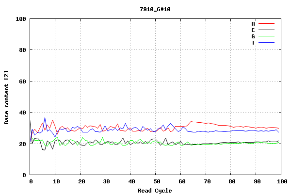
This plot shows the number of bases of each type (A, red; C, black; G, green; T, blue) sequenced during each sequencing cycle (out of 100 sequencing cycles, in this case). In this example, there are slightly more As and Ts sequenced than Gs and Cs, at each point.

Histogram of read qualities for forward and reverse reads
This plot has a histogram of qualities for forward and reverse reads. I think the lines represent different sequencing cycles, so the red line is cycle 1, the next line is cycle 2, and so on up to cycle 100, as we had 100 sequencing cycles in this example [is this right?] I'm not sure if this is average base qualities in reads, or mapping quality of reads (?). I think it must be base qualities.
Plot of read quality versus sequencing cycle, for forward and reverse reads
This plot shows the median (black line)), mean (red or green line) and interquartile range (grey area) of the qualities for forward and reverse reads (y-axes), versus the sequencing cycle (x-axis). I'm not sure if this is average base qualities in reads, or mapping quality of reads (?). I think it must be base qualities.
     We see that for the forward reads, the quality is low for the first ten cycles, then increases, and then decreases again slightly for the last 10-15 cycles. This is also seen for the reverse reads.
Here's one that looks pretty bad, it looks like the quality went down a lot during the sequencing cycles:

Plot of insertions and deletions versus sequencing cycle:
This plot shows the count of insertions (red line) and deletions (black line) versus the sequencing cycle (on the x-axis). Presumably this was estimated for some spiked DNA, for which the sequence was already known.
     We see that in this example the amount of insertions and deletions is fairly low for the first ten sequencing cycles, then increases, but stays steady until the last ten cycles, when there is a peak in indels.

Plot of log(indels) versus indel length:
This plot shows the log of the number of indels seen, versus the length of the indels in base-pairs, for insertions (red line), deletions (black line) and insertions plus deletions (green line). We see that there is not much difference in the pattern for insertions compared to deletions. For both, there are mostly smaller indels seen, and few large indels of >20 bp.

Plot of the number of mismatches versus the sequencing cycle:
This gives the number of mismatches (compare to the assembly used in the QC analyses, presumably) versus the sequencing cycle. Different plots are drawn for base positions at mismatches with base qualities of >30 (red), base qualities of 15-30 (green), >=15 (blue) and Ns (purple).
     Overall there seem to be most mismatches for the first 10 cycles, and for the last 10-15 cycles. We see that there are more base positions with lower qualities (green or blue) for later sequencing cycles than for early ones, although the first ten sequencing cycles also have quite a few low quality bases at mismatch positions (green).
Histogram of coverage:
This plot shows a histogram of coverage at the base positions for which we have mapped reads (mapped 'QC reads'). Here we see that the coverage ranges from 1 to about 37.
Plot of quality versus sequencing cycle:
This shows the quality versus sequencing cycle, for forward reads and reverse reads. I'm not sure if this is average base qualities in reads, or mapping quality of reads (?). I think it must be base qualities. I think this is the same as the lines for the mean values in 'Plot of read quality versus sequencing cycle, for forward and reverse reads' (see above).
Here's one that seems to have gone wrong, where the quality seems to have gone down a lot during the sequencing cycles, particularly for reverse reads:
Plot of mapped depth versus percentile of mapped sequence ordered by GC content:
On the x-axis we have the percentile of mapped sequence, ordered by GC content. For each percentile, we have the median mapped depth (blue line), the interquartile range of mapped depth (blue area), and the 10-90th percentile of mapped depth (grey area).
      In this example, the mapped depth increases with the percentile of mapped sequence, so seems to increase with the GC content. That is, there seems to be a greater median depth for higher-GC content than for lower GC content. This is a little worrying, as it suggests that there was more efficient mapping for high-GC sequences.


NPG stats
An alternative to QCGrind is NPG stats. For example, if the link to a QCGrind page is:
and the link to a liane in NPG stats is:

Tuesday 9 July 2013

Finding peaks in ChIP-Seq or FAIRE-Seq data using MACS

The MACS software can be used to identify peaks in ChIP-Seq data. It can also be used for other similar data such as FAIRE-Seq data, although it was designed for ChIP-Seq data.

Running MACS
To run it, you type this:
% macs14 -t /nfs/users/nfs_s/sh23/ChIP_seq_data/Antib.sorted.bam -c /nfs/users/nfs_s/sh23/ChIP_seq_data/input_sorted.bam -f BAM -g 350000000 -n test-ChIP
where -t  /nfs/users/nfs_s/sh23/ChIP_seq_data/Antib.sorted.bam specifies the ChIP-Seq data,
-c /nfs/users/nfs_s/sh23/ChIP_seq_data/input_sorted.bam specifies the control data,
-f BAM gives the format of the input files (BAM here),
-g 350000000 gives the effective genome size (350,000,000 for Schistosoma mansoni, as its genome is 350 Mb).
I submitted this job on the Sanger farm with 5 Gbyte of RAM.

Output files
An output file is made called test-ChIP_peaks.bed that has the positions of peaks identified.

bigger_blast.pl

This is of interest to Sanger users only.

Update: October 2013: farm_blast 
Martin Hunt has replaced bigger_blast.pl and blast_splitter.py with farm_blast.
For example:
% farm_blast -p blastp seq_update.fasta Bm.protein.fa --outdir inv_output 
which runs blastp using Bm.protein.fa as the query file, seq_updata.fasta as the database fasta file, and puts the results in output directory inv_output (which shouldn't exist beforehand). This doesn't need to be b-subbed, it will b-sub the jobs itself.

By default, farm_blast requests 500 Mbyte of memory. To request 1000 Mbyte (1 Gbyte), you can type:
% farm_blast -p blastp seq_update.fasta Bm.protein.fa --outdir inv_output --blast_mem 1.0

Farm_blast gives m8 format. The columns for m8 format are:
query id, subject id, % identity, alignment length, mismatches, gap opens, q. start, q. end, s. start, s. end, evalue, bit score

Another thing to know about farm_blast is that by default it splits up large sequences into chunks of 500000 bp. You can change the chunk size using the --split_bases option.

Running blast yourself 
You can run blast yourself by typing:
% makeblastdb -in mydb.fa -input_type fasta -dbtype prot
This formats a protein fasta file mydb.fa as the blast database.
Then run blast:
% blastp -query myquery.fa -db mydb.fa -task blastp -outfmt 6 -seg yes
This runs blastp between myquery.fa and database mydb.fa.
If you want SEG to be run, include '-seg yes' (the default is no SEG filtering).

Note: for blastn you can run '-dust yes' instead of '-seg yes'.


Now the rest of this blog (below) is obsolete, so I've changed it to pale grey.

--------------------------------------------------------------------------------------------------------------------------

Bigger_blast.pl
The path-dev group at Sanger have a script called bigger_blast.pl, that can be used to run blast jobs in parallel. You can get all the command-line options by typing:
% bigger_blast.pl
It can be run for example by typing:
% bigger_blast.pl -x -o myout2 /data/blastdb/Supported/nr my.fa
where -x selects blastx, -o specifies a prefix for the output file, /data/blastdb/Supported/nr is the database to run blast against, and my.fa is the query file.

The output files will be called myout.crunch.gz and myout.tab.gz. 

The myout .crunch.gz was produced using 'MSPcrunch -d' (ie. a crunch format file, although bigger_blast.pl doesn't use MSPcrunch to make it), and will look like this (you can look at it by typing 'gunzip -c myout .crunch.gz'):
72 49 11 81 SRAE_2000357600.t1:mRNA 2 72 E2AMU5.1 E2AMU5_CAMFO Histone-lysine N-methyltransferase SETMAR (Fragment)
70 48 13 83 SRAE_2000357600.t1:mRNA 22 92 E2BZV4.1 E2BZV4_HARSA Histone-lysine N-methyltransferase SETMAR (Fragment)
70 43 8 83 SRAE_2000357600.t1:mRNA 260 335 D2WLV0.1 D2WLV0_AGRPL Transposase
67 43 10 83 SRAE_2000357600.t1:mRNA 132 205 F4WLV9.1 F4WLV9_ACREC Histone-lysine N-methyltransferase SETMAR
67 45 10 83 SRAE_2000357600.t1:mRNA 20 93 E2C0B8.1 E2C0B8_HARSA Histone-lysine N-methyltransferase SETMAR (Fragment)

. . .
The myout.tab.gz is an EMBL feature table with one feature per hit. 

[Note: bigger_blast.pl doesn't run on farm3 yet.]

Running blastp
To run blastp, use '-p' instead of '-x'.

Setting the queue
To set the farm queue, use the '-q' option, eg.
% bigger_blast.pl -q yesterday -x -o myout2 /data/blastdb/Supported/nr my.fa

Setting the number of jobs to run
By default, bigger_blast submits 16 jobs. To submit more, use the '-j' option, eg.
% bigger_blast.pl -j 100 -x -o myout2 /data/blastdb/Supported/nr my.fa


Making a MSPcrunch format filesfrom normal blast output:
You can also run blast normally and make a MSPcrunch format file by typing afterwards:
%  bigger_blast.pl blast_output.txt
This should take the output of your blast search and convert it to crunch format.


Alternative to bigger_blast.pl
An alternative to bigger_blast.pl is Martin Hunt's blast_splitter.py script. For example:
% blast_splitter.py --protein_ref --splitmem=7 test.fa uniprot.renamed.fa ./blast_splitter 250000 -e 0.05 -p blastp -m8
where test.fa is your query fasta file of proteins. Magdalena suggested to use the -splitmem=5 or -splitmem=7 option. This will make an output directory blast_splitter with a file 'all.blast' that has the blast output. The 250000 means that the test.fa file is split into smaller files of 250,000 residues (amino acids here) each, for running blast. The output from blast_splitter.py will be in a subdirectory (called 'blast_splitter' here), and is a file called 'all.blast'.

Wednesday 3 July 2013

Running the path-dev functional annotation pipeline

This is only of interest to Sanger users, as it's only available on the Sanger farm. The path-dev group (Jacquilline Keane's team) have made a script called annotate_bacteria for annotation of bacterial genomes. It is based on PROKKA and is tailored for bacteria, archaea and viruses. It works by taking an assembly as input and identifying ORFs with Prodigal, and predicting RNA genes using RNAmmer and Aragorn.

It then predicts the functions of ORFs, by running BLAST against a database of proteins from RefSeq and UniProt (by default these are bacterial, archaeal and viral proteins), and comparing to domain databases (PfamA, CDD), and also runs SignalP to predict signal peptides. It gives evidence codes on the description lines to give the sources of the functional annotations.

To run it you type: [on farm3]
% annotate_bacteria -a assembly.fa --dbdir /lustre/scratch108/pathogen/pathpipe/prokka --sample_name MyExample
where assembly.fa is your input assembly,  /lustre/scratch108/pathogen/pathpipe/prokka is the directory with the sequence databases to run BLAST against, and MyExample is the label to give to the job.

The output appears in a subdirectory called 'annotation'. There is a file called MyExample.tbl that contains a summary of the annotation, eg.
>Feature HelminthExample|SC|contig000001
1       1254    CDS
                        EC_number       3.4.24.76
                        inference       ab initio prediction:Prodigal:2.60
                        inference       similar to AA sequence:UniProtKB:Q47899
                        inference       protein motif:Pfam:PF01400.18
                        locus_tag       HelminthExample_00001
                        product Flavastacin precursor
                        product Astacin (Peptidase family M12A)
                        protein_id      gnl|SC|HelminthExample_00001


Notes:
- This runs fine on farm3, but not on farm2. 
- Prodigal does not seem to predict partial genes (lacking a start and/or stop codon).
- Contigs in your input assembly.fa that are <200 bp are discarded.
- The RNA gene prediction step takes a long time.
- If you want to run a particular version of interproscan, you can do this with the -e option, eg. -e /software/pathogen/external/apps/usr/local/iprscan-5.0.7/interproscan.sh

Merging pdfs with pdftk

As discussed on Noel O'Blog's website, you can merge pdfs with the program pdftk.

For example, to merge three pdfs MolBiolCellCh1_fig1.pdf, MolBiolCellCh1_fig2.pdf and MolBiolCellCh1_fig3.pdf, you can type:
% pdftk A=MolBiolCellCh1_fig1.pdf B=MolBiolCellCh1_fig2.pdf C=MolBiolCellCh1_fig3.pdf  output MolBiolCellCh1_1_figs.pdf

This makes one output pdf, MolBiolCellCh1_1_figs.pdf, that has the three other pdfs merged together in order.

Monday 1 July 2013

Running a perl script with a particular version of Perl

If you want to use a perl script that only appeared in a particular version of perl (eg. the 'say' command, which appeared in perl 5.10), then you can specify inside the script that you can specify in the perl script that you want to use perl5.10 and that new features (such as 'say') should be enabled:

#!/usr/local/bin/perl
use 5.010;
say 'Hello';


Then you need to run the perl script with the correct version of perl for it to work:
% /software/perl-5.10.1/bin/perl -w my.pl
Hello

Note that if you don't use the correct version of perl, you'll get an error message:
% perl -w my.pl
Perl v5.10.0 required--this is only v5.8.8, stopped at my.pl line 3.
BEGIN failed--compilation aborted at my.pl line 3.


Note also that if you don't include the "use 5.010" in your script, it won't enable new features specific to 5.010 by default, and you'll get an error message because the 'say' command won't be recognised:

#!/usr/local/bin/perl
say 'Hello';


% /software/perl-5.10.1/bin/perl -w my.pl
Unquoted string "say" may clash with future reserved word at my.pl line 3.
String found where operator expected at my.pl line 3, near "say 'Hello'"
    (Do you need to predeclare say?)
syntax error at my.pl line 3, near "say 'Hello'"
Execution of my.pl aborted due to compilation errors.

Perl - getting a list of files in the current directory

To get a list of the names of files in a directory in Perl, you can use the glob function. This is what the book Effective Perl Programming suggests:

while (defined (my $file = glob('*') ) )
{
   do_something($file);
}

Here it is necessary to use 'defined', in case the name of the file is '0' (zero), which would appear to be false in the while loop, and cause the loop to terminate early.