Using mash to compare genome assemblies

I wanted to compare a set of 390 bacterial genome assemblies (for the bacterium Vibrio cholerae) to a set of 1664 genome assemblies, to see if there are any assemblies that are identical (or almost identical) between the two sets.

My colleagues in the Thomson group at Sanger mentioned the software Mash to me for this, which was published by Ondov et al 2016. 

Mash reduces large sequences and sequences sets (e.g. a genome assembly) to small, representative 'sketches', from which global mutation distances can be rapidly estimated. To create a sketch, each k-mer in a sequence is hashed. When 'mash sketch' is run, it automatically assesses the best k-mer size to use (see here for details). Sketches of different sizes can be compared using 'mash dist'.

There is a nice documentation for mash online.

Loading mash

To run mash, first I loaded the mash software (only necessary at Sanger):

% module avail -t | grep mash
mash/2.1.1--he518ae8_0
% module load mash/2.1.1--he518ae8_0

 

Creating sketches

Then,  I created 'sketches' for the set of 1664 genome assemblies (which all ended in *.fas), using a shell script like this:

#!/bin/sh
for i in `ls *.fas`
do
    echo "$i"
    mash sketch $i
done

This ran fine, and took about 35 minutes to run for the 1664 bacterial genome assemblies. This created a .msh (sketch) file for each of the assembly (.fas) files.

 

I then ran a similar script to create sketch files for the set of 390 genome assemblies.

Looking at the information on a sketch file

You can look at the information on a sketch file by typing something like:

% mash info THSTI_V12.contigs_spades.fasta.msh

You will see something like:
 Header:
  Hash function (seed):          MurmurHash3_x64_128 (42)
  K-mer size:                    21 (64-bit hashes)
  Alphabet:                      ACGT (canonical)
  Target min-hashes per sketch:  1000
  Sketches:                      1

Sketches:
  [Hashes]  [Length]  [ID]                            [Comment]

  1000      4042874   THSTI_V12.contigs_spades.fasta  [43 seqs] .THSTI_V12.1  [...]

Comparing genome assemblies using mash

Next, I compared pairs of genome assemblies (one from the set of 1664 assemblies versus one from the set of 390 assemblies), using mash, e.g.

% mash dist W2_T6.fasta.msh W1_T1.fasta.msh
W2_T6.fasta     W1_T1.fasta     0.000830728     0       966/1000
The results are tab delimited lists of Reference-ID, Query-ID, Mash-distance, P-value, and Matching-hashes. So, in the example above, the mash distance is 0.000830728.

 

Combining lots of sketch files using 'mash paste'

If you have a lot of sketch files, you may want to combine them using 'mash paste' into one large sketch file. You can do this as long as they have the same k-mer (you can find out their k-mer using 'mash info'; see above). 

 

For example, I had 1664 *msh files with a kmer size of 21. I first made a file with the list of all these .msh files:

% ls *msh > 1664_msh_files

Then I combined them into one large sketch file called 'combined.msh' by typing:

% mash paste combined -l 1664_msh_files

 

I wanted to compare these 1664 msh files to another set of 390 msh files. So I made a combined msh file using 'mash paste' for the 390 msh files. Then I can compare the combined msh file for the set of 1664 assemblies, to the combined msh file for the set of 390 assemblies, by running 'mash dist' on the two combined sketch files. Note that this is MUCH FASTER than using 'mash dist' to compare each of the 390 msh files for the first set of assemblies, to each of the 1664 msh files for the second set of assemblies!

 

 

Calculating assembly statistics

 [Note: this is useful to Sanger users only.]

There is a nice program called 'assembly-stats' for calculating assembly statistics on the Sanger farm. 

Find the latest version of it:

% module avail -t | grep -i stats
assembly-stats/1.0.1

Load the module:
% module load assembly-stats/1.0.1

Now run it on an assembly file '2038_EDC_717.fas':

% assembly-stats -t 2038_EDC_717.fas
filename        total_length    number  mean_length     longest shortest        N_count Gaps    N50     N50n    N70     N70n    N90     N90n
2038_EDC_717.fas        3816803 82      46546.38        362749  1020    2       1       163759  8       89245   15      24898   30

If you have a whole directory of assembly files all ending in '.fas', you can make a bourne-shell script to run assembly_stats on them, with a for loop:

#!/bin/sh

# see https://alvinalexander.com/blog/post/linux-unix/bourne-shell-script-for-loop-edit-files/
for i in `ls *.fas`
do
    echo "$i"
    assembly-stats -t $i > $i.stats
done

This makes a file .stats for each assembly file (e.g. 2038_EDC_717.fas.stats for assembly file 2038_EDC_717.fas).

Genome Decomposition Analysis (GDA)

 I have been using the Genome Decomposition Analysis (GDA) software by Eerik Aunin and Adam Reid to analyse the genome of the flatworm Schistosoma mansoni. 

 GDA is a new tool that is described in a paper by Aunin, Berriman and Reid (see here).

GDA extracts genomic features (e.g. gene density, repeat density, histone modification peaks, etc.) from sliding windows across chromosomes, and then clusters the genomic windows by similarity using HDBSCAN within GDA.

It is very useful for exploring trends across a genome.

I've included some instructions here on how to install and run GDA. However, the latest instructions and many more details can be obtained from the github page for GDA by Eerik Aunin and Adam Reid at Sanger: see https://github.com/eeaunin/gda.

Installing GDA

[Note to self: I did this on the Sanger farm.] 

I installed GDA using the following steps:

First I cloned the GDA git repository: [Note that I used the Sanger git repository; you probably need to use the git repository https://github.com/eeaunin/gda.]

% git clone https://gitlab.internal.sanger.ac.uk/ar11/gda.git

Then I ran the conda installation script:

% python gda/create_gda_conda_env.py gda_env gda_downloads gda

Then I activated the conda environment:

 % conda activate gda_env

Running GDA

Here is how I ran GDA for the test data set which comes with it, which is for Plasmodium falciparum:

First I ran the feature extraction pipeline:

% bsub -n12 -R"span[hosts=1]" -M10000 -R 'select[mem>10000] rusage[mem=10000]' -o gda_test.o -e gda_test.e "gda extract_genomic_features --threads 12 --pipeline_run_folder gda_pipeline_run gda/test_data/PlasmoDB-49_Pfalciparum3D7_Genome.fasta"

The output results were in the folder gda_pipeline_run.

Next I clustered the genome windows and analysed clusters:

% bsub -n1 -R"span[hosts=1]" -M10000 -R 'select[mem>10000] rusage[mem=10000]' -o gda_clustering_test.o -e gda_clustering_test.e "gda clustering -c 100 -n 5 gda_pipeline_run/merged_bedgraph_table/PlasmoDB-49_Pfalciparum3D7_Genome_merged_bedgraph.tsv"

The clustering output is in the folder gda_out. This is the output file that I can then use as input into the GDA Shiny app or IGV (see below). 

Using the GDA Shiny App

[Note to self: I did this on my Mac laptop rather than on the Sanger farm.]

There is a lovely Shiny App for viewing the GDA results.

To install the Shiny App, I first downloaded the GDA code using:

% git clone https://gitlab.internal.sanger.ac.uk/ar11/gda.git

To install the Shiny App in R, I typed (in R):

> source("gda/gda_shiny/install_gda_shiny_dependencies_without_conda.R")

Then I can start the Shiny App using:

% python3 gda/gda_shiny/gda_shiny.py gda_out_mydata_1kb

where gda_out_mydata_1kb is my output directory from running GDA.

This starts the Shiny App in my browser and I get lovely pictures like this UMAP plot showing the GDA clusters:

 

 

The Shiny App also gives many other nice outputs, for example a heatmap showing input variables for the GDA clusters; a plot showing distribution of GDA clusters across the chromosomes; and a table showing the variables that are significantly different for each particular GDA cluster compared to the other clusters.

Viewing GDA results in the IGV genome browser:

[Note to self: I did this on my Mac laptop rather than on the Sanger farm.]

To view the results from GDA in the IGV genome browser, you first need to install the IGV software by following the instructions on the IGV website here.

To load the GDA results into IGV,  as well as the bedgraph files of features that GDA used as input, you need to run something like this:

% gda/gda_make_igv_session_file.py -g schistosoma_mansoni.PRJEA36577.WBPS14.annotations.gff3 gda_out_mydata_1kb/cluster_heatmap.csv gda_out_mydata_1kb/schisto_v7/clusters.bed schistosoma_mansoni.PRJEA36577.WBPS14.genomic.fa bedgraph_output_mydata

where schistosoma_mansoni.PRJEA36577.WBPS14.annotations.gff3 is the file with the annotations of genes, mRNAs, etc. for your genome;

gda_out_mydata_1kb is the folder containing the output from your GDA run;

bedgraph_output_mydata is the folder with input bedgraph files used as input for GDA.

This will make a file igv_session_gda.xml.  

Then start up IGV [Note to self: I have the IGV icon on my desktop on my laptop.]

Then if you start up IGV you can go load this file into IGV by going to File->Open session, and then choose 'igv_session_gda.xml' as the session file. 

It may be a little slow to load all the data into IGV, but you can look at the bottom right of the IGV screen to see it is loading data (it will say things like '1317M of 2359M', etc.).

Once it has loaded, you can view the GDA clusters along the bottom of the screen, as well as all the inputs that were used for GDA above that (e.g. GC content, genes, UTRs, etc.):

 

 

 

Acknowledgements

A big thank you to Eerik Aunin and Adam Reid for helping me with running GDA.

 

 

Exporting protein sequences from Artemis

 I had a gff with the annotation and genome sequences for some contigs, and wanted to export the protein sequences from Artemis. I wrote previously on how to run Artemis here but that was ages ago, so had to remind myself!

To log into the Sanger compute cluster and run Artemis:

% ssh -Y pcs6

% module avail -t | grep -i art

% module load artemis/18.1.0

% art

This then opened Artemis, and to load my gff file, I used the 'File' menu. 

Then to select my genes of interest, I went to the 'View' menu, and choose 'CDS genes and products', and then went to the 'Select' menu and chose 'All CDS features', and chose my genes of interest from the list. Then I went to the 'Write' menu and chose 'Amino acids of selected features to file', and this wrote a file with the protein sequences for my genes of interest. Great!

Exploring Vibrio cholerae data in Pathogenwatch

Today I've been exploring the Vibrio cholerae (the bacterial species that causes the disease cholera) genome data available in the Pathogenwatch website.

Finding out how many Vibrio cholerae genomes are in Pathogenwatch

I went to the Pathogenwatch website and clicked on 'Genomes' at the top. At the top, it says 'Viewing 73,294 of 73,294 genomes', which is all the genomes in Pathogenwatch for all species. To select V. cholerae genomes, I selected 'Vibrio' in the 'Genus' list on the left, and this then gave me a list of 390 V. cholerae genomes in a table:

 

 

There are several columns in the table:
Name: name of the assembly for the strain/isolate.

Organism:  this is Vibrio cholerae in all cases.

Type: this is the group that this strain/isolate is classified into, using the MLST (multi-locus sequence typing) schema. The most common types are 69 (327 isolates/strains), followed by 737 (7 isolates/strains), 170 (5 isolates/strains), 48 (4 isolates/strains), 75 (3 isolates/strains), and so on.

Typing schema: this is MLST in all cases.

Country: this is the country that the strain/isolate was collected in (if available). The most isolates come from Mexico (92 isolates/strains), followed by China (59), Haiti (34), Nepal (25), India (20), Bangladesh (16) and Brazil (11), and so on. There are 57 strains/isolates with no country available, so we only have country information for 333 strains/isolates.

Date: this is the date the strain/isolate was collected (if available). These range from 1930 to 2011.

Access: this has values 'Public' or 'Reference'. I think the 'Reference' cases are reference genomes, and the rest are strains collected around the world. 

 

The genomes listed as 'Reference' for V. cholerae are:

(1) Env-seawater, collected in 1982 in Brazil, with MLST type 79,
(2) Env-sewage, collected in 1978 in Brazil, with MLST type 48,

(3) 7PET_MiddleEastern, with MLST type 69,

(4) M66, with MLST type 71,

(5) W1_T1, with MLST type 69,

(6) W1_T2, with MLST type 69,

(7) W1_T3, with MLST type 69,

(8) W1_T4, with MLST type *b5a7,

(9) W1_T5, with MLST type 69,

(10) W1_T6, with MLST type 69,

(11) W1_T7, with MLST type 69,

(12) W1_T8, with MLST type 69,

(13) W1_T9, with MLST type 69,

(14) W1_T10, with MLST type 69,

(15) W1_T11, with MLST type 69,

(16) W1_T12, with MLST type 69,

(17) W1_T13, with MLST type 69.

I think that the MLST type *b5a7 for W1_T4 means that it didn't have a MLST type assigned, because the allele is not known for one of the loci.

Making a map for the sources of Vibrio cholerae genomes in Pathogenwatch

At the top of the list of 390 V. cholerae genomes, there are there three links, 'List', 'Map', 'Stats'. If you click on the 'Map', it gives you a map of where all the V. cholerae isolates/strains came from in the world:

 

You can see on the map that there are 92 isolates/strains from Mexico, 59 from China, 34 from Haiti, 25 from Nepal, 20 from India, 16 from Bangladesh, 11 from Brazil, and so on.

 

Getting assembly statistics for the Vibrio cholerae genomes in Pathogenwatch

If you click on the 'Stats' link at the top of the page (from the three links 'List', 'Map', 'Stats'), you will get assembly statistics for the 390 Vibrio cholerae genomes. There are several different assembly statistics available: genome length, N50, number of contigs, non-ACTG bases, and GC content.

 

If we look at the genome length, we see that the average genome size is 4,021,504.5 bases, about 4 Mbases:

 

 

I have labelled a couple of the assemblies that seem to have an unusually large or small assembly size. These might possibly be misassemblies, I think. In particular, the assembly SRR221551.contigs_spades seems to be huge (about 6.7 Mbases) compared to the rest.

 

If we look at the number of contigs,  we see most assemblies have about 75 contigs (average 73.9), but that assembly SRR221551.contigs_spades also has a very large number of contigs, again suggesting the assembly is a bit dodgy:

Again, when we look at the GC content, we see that the assemblies have an average GC content of 47.5%, but assembly SRR221551.contigs_spades looks strange as it has an average GC content of about 53%: 

 

 

Investigating the Haiti outbreak of Vibrio cholerae in Pathogenwatch

We can investigate the Haiti outbreak of Vibrio cholerae by creating a 'collection' of the V. cholerae isolates from Haiti in Pathogenwatch. I think that you need to log into Pathogenwatch using an email address to be allowed to do this. Then, in the 'map' view of all V. cholerae isolates from around the world, use the 'map selection tool' to draw a shape around Haiti, and this then selects the 34 V. cholerae isolates from Haiti:

 

 

 

 

 

In the list of assemblies that appears from Haiti (list on the left), select all the assemblies from Haiti, and then click on the 'Select genomes' button on the right and choose 'Create collection'. (Note: for some reason, I don't always see the 'Create collection' button, I'm not sure why.)

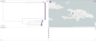
You can now see in the 'Collection view', that there is a map at the top showing Haiti, and a timeline at the bottom showing the dates for the isolates. In this case they are all for 2010. If you click on 'View tree', it will show a tree of the Haiti isolates also, which is a neighbour-joining tree based on the 'core' genes:

 

 

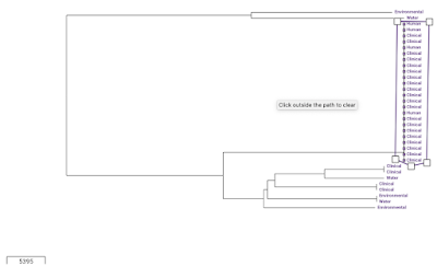
We can view the metadata for the assemblies in the collection by clicking on the 'Timeline' button at the bottom, and selecting 'Metadata' instead of 'Timeline'. One of the variables in the Metadata for the Haiti isolates is 'Source', which can take values such as 'Clinical', 'Environmental', and 'Water'. To show the 'Source' variable on the tree', we click on the 'Source' column in the Metadata table. Then click on the 'Settings' icon in the tree, and in the 'Nodes and labels' menu at the top left, we select 'Show leaf labels'. Note that the tree is a bit hard to read because the nodes are so big; to make them smaller click on the 'Nodes and labels' menu, and reduce the node size. We can see that there is one clade (which I've drawn a box around) of identical (or near identical) sequences that consists only of human/clinical isolates:

 

 

 

 

 

 

 

 

 

 

 We can also view the MLST typing information for the isolates by selecting 'Typing' instead of 'Metadata'/'Timeline' in the menu on the bottom left. If we click on the 'Biotype' column, it shows in the tree that the highlighted clade all has the 'O1 pathogenic' biotype:

 

 

 

 

 

 

 

 

 

 

If we choose to display 'Reference' from the 'Typing' columns, we see that the isolates in this clade are closest to the W3_T12 reference, while the other isolates are closest to the 'Env_Sewage' reference:

 

 

 

 

 

 

 

 

 

 

 

 

 

And, if we choose the 'ST' column (MLST), we can see that the isolates in this clade are the 69 type, while the other isolates in the clade have a variety of MLST types:

Another interesting thing to look at is antibiotic resistance, and to do this we choose the 'Antibiotics' (instead of 'Timeline'/'Typing'/etc.). We should then see a table below with the resistance to different antiobiotics, with red dots indicating resistance:

 

As before, we can select a column, e.g. chloramphenicol resistance, and show which isolates are predicted to have chloramphenicol resistance on the tree, and we see that it is just the 'O1 pathogenic' clade that is predicted to have chloramphenicol resistance:

Using Weblogo for sequence logos

A very nice tool for creating sequence logos is the Weblogo website.
You can paste in a multiple alignment like this:

AATGGAAGTGGAAAATCTGTTAGCA
TTATATTAGGAAAATCGTTATAGCA
ATTATGAGTGGAAAATCATGTAGCA
GAAATCAATTGATAGAATATGAGCA

and get back a sequence logo, lovely!

 

 

 

Using Ontologizer for GO enrichment analysis

I previously used the Ontologizer tool for GO enrichment analysis, but that was a few years ago (see Woods et al PMID:23675306). I remember it having a nice algorithm that takes the relationship between parent and child GO terms into account. I decided to use it again, this time to test for GO enrichment among a list of Schistosoma mansoni genes.  

Installing Ontologizer

I downloaded Ontologizer onto the Sanger compute farm using:

% wget http://ontologizer.de/cmdline/Ontologizer.jar 

This is the command-line version of Ontologizer.

You can see instructions for installing it and running it here: here.

Note I remember there was also a beautiful GUI for Ontologizer. There are instructions for installing it here. However, unfortunately I wasn't able to figure out how to install it this time (I tried to install on my Mac laptop, and found it needs a file swt.jar, which I wasn't able to find on the web, the links to that seem to be broken now.) Oh well!

Preparing the inputs for Ontologizer 

First I downloaded the Gene ontology hierarchy file using:

% wget http://purl.obolibrary.org/obo/go/go-basic.obo

Next I wanted to get the GO annotations for Schistosoma mansoni. There are not curated annotations on the GO downloads page, so I used BioMart in WormBase ParaSite to get a set of predicted GO annotations:

- I went to BioMart in WormBase ParaSite

- For the Query, I chose the genome to be Schistosoma mansoni

- I selected the Output attributes to be GO: GO term accession, GO term name, GO term definition, GO term evidence code, GO domain

- I clicked on 'Results' at the top of the webpage

- I clicked on 'Export as CSV' and got the file 'mart_export.txt', which I renamed as 'smansoni_biomart.txt'

 

For Ontologizer, the annotations need to be in a format called GAF format. I wrote a little perl script make_gaf.pl  to convert the file 'smansoni_biomart.txt' to GAF format:

% perl -w make_gaf.pl smansoni_biomart.txt  > smansoni.gaf

Here is my perl script make_gaf.pl:

 

#!/usr/local/bin/perl

# read in the GO data for S. mansoni from WormBase ParaSite Biomart:
$go_data = $ARGV[0]; # smansoni_biomart.txt

# Genome project,Gene stable ID,GO term accession,GO term name,GO term definition,GO term evidence code,GO domain
# schistosoma_mansoni_prjea36577,Smp_000020,,,,,
# schistosoma_mansoni_prjea36577,Smp_000030,GO:0000502,proteasome complex,"A large multisubunit complex which catalyzes protein degradation, found in eukaryotes, archaea and some bacteria. In eukaryotes, this complex consists of the
barrel shaped proteasome core complex and one or two associated proteins or complexes that act in regulating entry into or exit from the core.",IEA,cellular_component
# schistosoma_mansoni_prjea36577,Smp_000030,GO:0042176,regulation of protein catabolic process,"Any process that modulates the frequency, rate or extent of the chemical reactions and pathways resulting in the breakdown of a protein b
y the destruction of the native, active configuration, with or without the hydrolysis of peptide bonds.",IEA,biological_process
# schistosoma_mansoni_prjea36577,Smp_000030,GO:0030234,enzyme regulator activity,Binds to and modulates the activity of an enzyme.,IEA,molecular_function
# schistosoma_mansoni_prjea36577,Smp_000030,GO:0050790,regulation of catalytic activity,Any process that modulates the activity of an enzyme.,IEA,biological_process

print "!gaf-version: 2.1\n";
open(GO,"$go_data") || die "ERROR: cannot open $go_data\n";
while(<GO>)
{
    $line = $_;
    chomp $line;
    if (substr($line,0,3) eq 'sch' && $line =~ /GO:/)
    {
        @temp = split(/\,/,$line);
        $gene = $temp[1]; # e.g. Smp_000030
        $term = $temp[2]; # e.g. GO:0000502
        $evid = $temp[$#temp-1]; # e.g. IEA
        $type = $temp[$#temp]; # e.g. biological_process
        if    ($type eq 'biological_process') { $type = 'P';}
        elsif ($type eq 'molecular_function') { $type = 'F';}
        elsif ($type eq 'cellular_component') { $type = 'C';}
        # Note: S. mansoni has taxon_id 6183 in the NCBI Taxonomy: https://www.ncbi.nlm.nih.gov/Taxonomy/Browser/wwwtax.cgi?id=6183
        # Column 1: DB                 :  required=1   e.g. UniProtKB or WormBase ParaSite
        # Column 2: DB Object ID       :  required=1   e.g. P12345
        # Column 3: DB Object Symbol   :  required=1   e.g. PHO3
        # Column 4: DB Object Qualifier:  optional     e.g. NOT
        # Column 5: GO ID              :  required=1   e.g. GO:0003993
        # Column 6: DB:Reference       :  required=1   e.g. PMID:2676709
        # Column 7: Evidence code      :  required=1   e.g. IMP
        # Column 8: With/From          :  optional     e.g. GO:0000346
        # Column 9: Aspect             :  required=1   e.g. F
        # Column10: DB Object name     :  optional     e.g. Toll-like receptor 4
        # Column11: DB Object synonym  :  optional     e.g. hToll
        # Column12: DB Object type     :  required=1   e.g. protein
        # Column13: Taxon              :  required=1   e.g. taxon:9606
        # Column14: Date               :  required=1   e.g. 20090118
        # Column15: Assigned By        :  required=1   e.g. SGD
        # Column16: Annotation extension: optional     e.g. part_of(CL:0000576)
        # Column17: Gene Product Form ID: optional     e.g. UniProtKB:P12345-2
        $gene_symbol = $gene."_symbol";
        $gene_alias = $gene."_alias";
        print "WB\t$gene\t$gene_symbol\tinvolved_in\t$term\tpubmed\t$evid\t\t$type\t\t$gene_alias\tgene\ttaxon:6183\t20211022\tWB\t\t\n";
    }
}
close(GO);

print STDERR "FINISHED\n";

The other things you need for Ontologizer are a list of your genes of interest, and a list of all genes (a background set). I had a list of all genes in the S. mansoni gene set as the background set (called 'all_schisto_v7'). The file with my list of genes of interest was called cluster0_genesB.

Running Ontologizer

I found that I was not able to run Ontologizer on the head node of the Sanger farm, so submitted it as a farm job. Here is the command I used:

% bsub -o cluster0_genes.o -e cluster0_genes.e -R "select[mem>1000] rusage[mem=1000]" -M1000 "/usr/bin/java -Xmx1G -jar Ontologizer.jar -g go-basic.obo -a smansoni.gaf -p all_schisto_v7 -s cluster0_genesB"

That is, the actual Ontologizer command was:

% java -jar Ontologizer.jar -g go-basic.obo -a smansoni.gaf -p all_schisto_v7 -s cluster0_genesB

 

This made an output file: table-cluster0_genesB-Parent-Child-Union-None.txt

The output file looks a bit like this:

 

ID      Pop.total       Pop.term        Study.total     Study.term      Pop.family      Study.family    nparents        is.trivial      p       p.adjusted      p.min   name
GO:0031224      10129   2072    1464    228     4152    290     2       false   1.797278481560433E-25   1.797278481560433E-25   0.0     "intrinsic component of membrane"
GO:0016020      10129   2345    1464    234     4152    290     1       false   2.0730394290778032E-19  2.0730394290778032E-19  0.0     "membrane"
GO:0017171      10129   60      1464    25      886     75      1       false   1.5850273023050352E-13  1.5850273023050352E-13  9.159281107768625E-95   "serine hydrolase activity"
GO:0006508      10129   346     1464    51      1247    82      1       false   1.471129482398609E-11   1.471129482398609E-11   6.0266E-319     "proteolysis"
GO:0008233      10129   250     1464    42      1321    89      2       false   2.535618270865147E-10   2.535618270865147E-10   1.6965153175154988E-277 "peptidase activity"
GO:0008289      10129   72      1464    16      3678    154     1       false   2.2267642693677877E-8   2.2267642693677877E-8   2.3266792066569023E-153 "lipid binding"
GO:0008236      10129   60      1464    25      250     42      2       false   4.6040476340954584E-8   4.6040476340954584E-8   2.491599802996095E-59   "serine-type peptidase activity"
GO:0004252      10129   52      1464    25      162     37      2       false   4.0367746142102156E-7   4.0367746142102156E-7   1.041762945213498E-43   "serine-type endopeptidase activity"
GO:1901564      10129   1438    1464    93      2479    118     2       false   9.21145381068937E-7     9.21145381068937E-7     0.0     "organonitrogen compound metabolic process"

...

 

By default, Ontologizer does not use any correction for multiple testing, so I wanted to correct for the fact that I was testing so many GO terms at once. I decided to use the Bonferroni correction:

% bsub -o cluster0_genes.o -e cluster0_genes.e -R "select[mem>1000] rusage[mem=1000]" -M1000 "/usr/bin/java -Xmx1G -jar Ontologizer.jar -g go-basic.obo -a smansoni.gaf -p all_schisto_v7 -s cluster0_genesB -m Bonferroni"

 

% head table-cluster0_genesB-Parent-Child-Union-Bonferroni.txt
ID      Pop.total       Pop.term        Study.total     Study.term      Pop.family      Study.family    nparents        is.trivial      p       p.adjusted      p.min   name
GO:0031224      10129   2072    1464    228     4152    290     2       false   1.797278481560433E-25   1.7595356334476639E-22  0.0     "intrinsic component of membrane"
GO:0016020      10129   2345    1464    234     4152    290     1       false   2.0730394290778032E-19  2.0295056010671693E-16  0.0     "membrane"
GO:0017171      10129   60      1464    25      886     75      1       false   1.5850273023050352E-13  1.5517417289566294E-10  9.159281107768625E-95   "serine hydrolase activity"
GO:0006508      10129   346     1464    51      1247    82      1       false   1.471129482398609E-11   1.4402357632682383E-8   6.0266E-319     "proteolysis"
GO:0008233      10129   250     1464    42      1321    89      2       false   2.535618270865147E-10   2.482370287176979E-7    1.6965153175154988E-277 "peptidase activity"
GO:0008289      10129   72      1464    16      3678    154     1       false   2.2267642693677877E-8   2.180002219711064E-5    2.3266792066569023E-153 "lipid binding"
GO:0008236      10129   60      1464    25      250     42      2       false   4.6040476340954584E-8   4.5073626337794536E-5   2.491599802996095E-59   "serine-type peptidase activity"
GO:0004252      10129   52      1464    25      162     37      2       false   4.0367746142102156E-7   3.952002347311801E-4    1.041762945213498E-43   "serine-type endopeptidase activity"
GO:1901564      10129   1438    1464    93      2479    118     2       false   9.21145381068937E-7     9.018013280664893E-4    0.0     "organonitrogen compound metabolic process"
 

More information on Ontologizer

It is also possible to produce some graphical output from the command-line version of Ontologizer, you can see details of that here.